Working with Waiwera output

Waiwera’s main simulation results are output to an HDF5 file, which may be configured via the JSON input file (see Simulation output).

Viewing simulation output

Various software tools are available for viewing the groups and datasets in HDF5 files. The simplest is h5dump, a command-line tool which can dump an ASCII representation of the HDF5 file’s contents to the console.

There are also graphical tools for viewing HDF5 files, for example HDFView, Silx (see Fig. 9) and others. These tools typically also include features for producing simple plots of the datasets.

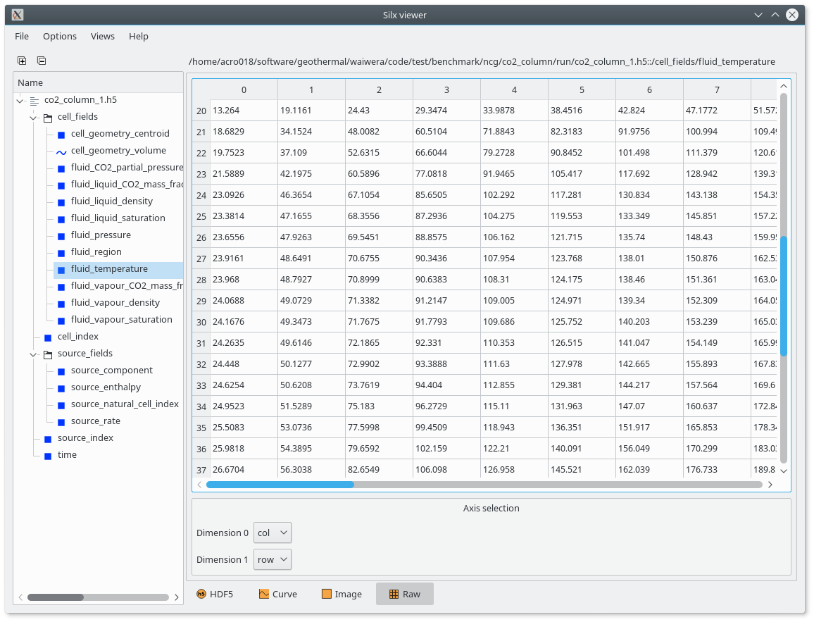
Fig. 9 Viewing a Waiwera HDF5 output file with Silx viewer

How simulation output is structured

Data in HDF5 files are generally organised into groups, which may be considered analogous to directories in a file system. A group may contain one or more datasets. All the groups and datasets in an HDF5 file are contained in a top-level group called the “root” group. For more information on the HDF5 data model, refer to the HDF5 documentation.

Under the root group, a Waiwera HDF5 output file usually contains two groups, “cell_fields” and “source_fields”. Two other groups, “face_fields” and “minc”, may also be present, depending on how the simulation is configured. The contents of these four groups is described below, along with other datasets which may be present in the root group.

Output at cells

The “cell_fields” group in a Waiwera HDF5 output file contains output data defined at the cells. The main datasets in this group contain the fluid properties computed in the cells. These datasets have names beginning with “fluid_” (e.g. “fluid_liquid_density”). The specific fluid datasets included here can be selected in the Waiwera JSON input file (see Fluid fields).

Because the fluid datasets are generally time-dependent, there is one row in the dataset for each output time (see Output time dataset), and on each row there is one column per cell.

The “cell_fields” group also contains datasets related to cell geometry, which have names beginning with “cell_geometry”. For example, the “cell_geometry_volume” dataset contains the volumes of all the cells. These datasets are not time-dependent, so there is just one row per cell. The “cell_geometry_centroid” dataset contains a three-element array for each cell, so there are three columns on each row.

If tracers are being simulated (see Tracers), then the “cell_fields” group also contains datasets for the tracer mass fractions, one dataset for each tracer. The names of these datasets are “tracer_” followed by the tracer name. These datasets are automatically included whenever tracers are simulated.

Output at sources

The “source_fields” group in a Waiwera HDF5 output file contains output data defined at the sources (see Source terms), for example the flow rate and enthalpy at each source. These datasets have names beginning with “source_”, e.g. “source_rate”. The datasets included here can be selected in the Waiwera JSON input file (see Source fields).

Like the fluid datasets, most of the source datasets are time-dependent, having one row per output time, with each row having one column per source.

If the simulation uses a source network (see Source networks), the “source_fields” group in the HDF5 output file also contains output data defined at the source network groups and reinjectors. These datasets have names beginning with “network_”, e.g. “network_group_rate”, “network_reinject_overflow_steam_rate”. The datasets included here can also be selected in the Waiwera JSON input file (see Source network fields). Again, most of the group and reinjector datasets are time-dependent, with one row per output time and each row having one column per group or reinjector.

Output at faces

The “face_fields” group in a Waiwera HDF5 output file contains output data defined at the mesh faces. The main datasets in this group contain fluid fluxes computed through the faces. These datasets have names beginning with “flux_” (e.g. “flux_water”, “flux_energy” or “flux_vapour”). The specific flux datasets included here can be selected in the Waiwera JSON input file (see Flux fields). Note that if no flux fields are specified for output (which is the default), the “face_fields” group will not be present.

As for the cell fields, the flux datasets are usually time-dependent, so there is one row for each output time (see Output time dataset), and on each row there is one column per face.

The “face_fields” group also contains datasets related to face geometry, which have names beginning with “face_geometry”. For example, the “face_geometry_area” dataset contains the face areas. These datasets are not time-dependent, so there is just one row per face. Some of the face geometry datasets (e.g. “face_geometry_distance”, “face_geometry_normal”, “face_geometry_centroid”) contain arrays for each face, so there are multiple columns on each row.

Output time dataset

The root group in a Waiwera HDF5 output file also contains a “time” dataset. This is a simple array containing all the output times, one per row. These rows correspond to the rows in time-dependent datasets in the “cell_fields”, “face_fields and “source_fields” groups.

Index datasets and data ordering

When PETSc writes cell data from a parallel simulation to HDF5 output, by default the data are not written in the original or “natural” ordering that would occur in a serial simulation. This is because in a parallel simulation, the mesh is distributed amongst the different parallel processes, and re-assembling the distributed data back into its natural ordering would require a parallel “scattering” operation every time data were to be output. Operations requiring parallel communication need to be kept to a minimum if the code is to scale well to large numbers of parallel processes.

Instead, data are written out in what is known as “global” ordering. Here, the data are written in process order, so all the data from parallel process 0 are written first, followed by all the data from process 1, and so on. On each process, the data are written out according to a “local” ordering on that process, which is generally not related to the natural ordering.

As an example, consider the simple 9-cell 2-D mesh in Fig. 10, and a possible partition of it amongst two parallel processes. In a serial simulation, cell data would simply be written out in the natural ordering, [0, 1, 2, … 8]. After the parallel partitioning, however, the natural indices corresponding to the local ordering on process 0 are [3, 6, 7, 8], and those on process 1 are [0, 1, 2, 4, 5]. Hence when cell data over the whole mesh are written out in parallel, the natural indices corresponding to the global output ordering are [3, 6, 7, 8, 0, 1, 2, 4, 5].

Fig. 10 Natural and local cell ordering

The Waiwera HDF5 output file contains a dataset (in the root group) called “cell_index” which is a mapping from the natural cell ordering onto the global cell ordering used in the output. Hence, if the “cell_index” dataset is represented by the array \(c\), then the index of the global cell data corresponding to natural index \(i\) is given by \(c[i]\). For example, the “cell_index” array for the mesh in Fig. 10 would be [4, 5, 6, 0, 7, 8, 1, 2, 3].

This index array can be used to re-order output in global output ordering back into natural ordering, for post-processing. It is also used internally by Waiwera to re-order fluid data when a simulation is restarted from the output of a previous run (see Restarting from a previous output file).

Similarly, there is another dataset called “source_index” which maps the natural source ordering onto the global source ordering in the output. The “natural” source ordering follows the order in which sources are specified in the input. If a source specification defines multiple sources using the “cells” array, the natural source ordering follows the specified cell order within that specification. If a source specification defines multiple sources using the “zones” value, the natural source ordering follows the natural cell ordering within each zone.

If a source network (see Source networks) is used in the simulation, there may be additional “network_group_index” and “network_reinject_index” datasets which map the natural source group and reinjector ordering (following the ordering in the input) to the global group and reinjector ordering in the output. (Note that even in a serial simulation, these global orderings may not be the same as the natural orderings, because groups and reinjectors may be internally re-ordered if, for example, a group in the input refers to other groups which are only defined later in the input.)

If there is Output at faces (in the “face_fields” HDF5 group) then two more index datasets will be present in the root group: “face_cell_1” and “face_cell_2”. These contain the natural indices of the cells on either side of each face, and can be used to identify the correct face field data for a given face in the simulation mesh.

Besides the internal mesh faces, the face field datasets also contain data for boundary faces on which Dirichlet boundary conditions are applied. These faces cannot be identified by a pair of natural cell indices, because there is no mesh cell on the outside of the boundary. Dirichlet boundary conditions are specified via the “boundaries” array value in the Waiwera JSON input file. Each item of this array specifies a different boundary condition. For boundary faces in the output, the “face_cell_1” dataset contains the natural index of the cell on the inside of the boundary, but the “face_cell_2” dataset contains the negative of the (1-based) index of the boundary condition specification in the input. Hence, for example, a boundary face with the first boundary condition applied to it has a “face_cell_2” value of -1, a face with the second boundary condition applied has a “face_cell_2” value of -2, etc.

MINC cell indexing

For MINC simulations, MINC matrix cells are added inside the corresponding fracture cells (see Modelling fractured media using MINC). Datasets in the “cell_fields” group contain results for all cells, including MINC matrix cells.

Extended natural cell indices

As MINC matrix cells are not present in the original mesh, they do not have a “natural” index. Hence, they must be assigned an “extended” natural index.

MINC matrix cells are added after the single-porosity and fracture cells (which retain the natural cell indices of the original mesh), and are added in order of MINC matrix level (all level 1 cells first, then level 2, etc.). Within each matrix level, matrix cells are added following the natural order of their associated fracture cells. The extended natural indexing of MINC cells corresponds to this order in which they are added to the mesh.

For MINC simulations, the “cell_index” dataset maps extended natural cell indices to the global cell ordering used in the output. The cell indices in the “face_cell_1” and “face_cell_2” datasets are also then extended natural indices.

Datasets in the “minc” group

Waiwera HDF5 output files from MINC simulations also contain an additional “minc” group. This contains two datasets to assist with post-processing the results of MINC simulations.

The “level” dataset contains the MINC level for each cell. For MINC matrix cells, this corresponds to the MINC matrix level. For example, for dual-porosity simulations each fracture cell has only one matrix cell inside it, so all matrix cells have level 1. If there are two MINC matrix levels, matrix cells will have levels 1 and 2, etc.

Fracture cells are assigned MINC level 0. If MINC is applied over only part of the simulation mesh, there will be single-porosity cells outside it, and these are assigned MINC level -1.

The “parent” dataset contains, for each cell, the natural index of its parent cell. For MINC matrix cells, the parent cell is the corresponding fracture cell. For fracture cells and single-porosity cells, the parent cell is just the cell itself.

Together, these two datasets can be used to identify the cell results corresponding to the MINC matrix cell of any level within a particular fracture cell.

Simulation output and scripts

For more complex post-processing tasks, there are libraries available for handling HDF5 files from a variety of scripting and programming languages (including C, C++, Fortran, Python, Java, Matlab, Mathematica and R).

For example, h5py is a Python library for interacting with HDF5 files. The Python script below uses h5py to open a Waiwera HDF5 output file and produce a plot of temperature vs. elevation for a vertical column model, at the last time in the file:

import h5py
import matplotlib.pyplot as plt

out = h5py.File('model.h5', 'r')

index = out['cell_index'][:,0]
z = out['cell_fields']['cell_geometry_centroid'][index, 1]
T = out['cell_fields']['fluid_temperature'][-1, index]

plt.plot(T, z, '.-')
plt.xlabel('Temperature ($^{\circ}$C)')
plt.ylabel('elevation (m)')
plt.show()

Note that after the file is opened, the “cell_index” array is read into the index variable. This is then used to re-order the elevation and temperature arrays, to make sure they are in natural ordering before plotting (see Index datasets and data ordering).

Here the second column (\(y\)-coordinate) of the centroid array is read in, to give the cell elevations (for a 2-D model). The rows of the temperature array represent different times, so the last row is read in to give the final set of results in the output. Finally, the results are plotted using the matplotlib plotting library (Fig. 11).

Fig. 11 Temperature vs. elevation plot from Waiwera HDF5 output

If the Layermesh library is used to create the Waiwera simulation mesh (see Creating meshes), it can also be used to produce 2-D layer and vertical slice plots of Waiwera results. For example, the following script produces plots of steady-state temperatures and vapour saturations along a vertical slice through the centre of the 3-D geothermal model created in Setting up simulations using scripts:

import h5py
import matplotlib.pyplot as plt
import layermesh.mesh as lm

mesh = lm.mesh('demo_mesh.h5')
results = h5py.File('demo.h5', 'r')
index = results['cell_index'][:,0]

T = results['cell_fields']['fluid_temperature'][-1][index]
S = results['cell_fields']['fluid_vapour_saturation'][-1][index]

fig = plt.figure(figsize = (5, 6))

ax = fig.add_subplot(2, 1, 1)
mesh.slice_plot('x', value = T, axes = ax,
                value_label = 'Temperature',
                value_unit = '$^{\circ}$C',
                colourmap = 'jet')

ax = fig.add_subplot(2, 1, 2)
mesh.slice_plot('x', value = S, axes = ax,
                value_label = 'Vapour saturation',
                colourmap = 'jet')

plt.savefig('results.pdf')
plt.show()

This script produces the plots below:

Fig. 12 Steady-state temperature and vapour saturation results for demo simulation

Log output

Log output is written to a log file, separate from the main HDF5 simulation output file. The log file is in YAML format, which is text-based, so it can be read with a text editor. As for the Waiwera JSON input file (see Waiwera input), using a programming editor with syntax highlighting can make reading YAML files easier. (For details on the structure of the log messages in the Waiwera YAML log file, see Log message structure.)

For more complex post-processing tasks, libraries are also available for handling YAML files in various programming and scripting languages. For example, PyYAML is a library for handling YAML files via Python scripts. The following Python script uses PyYAML to read a Waiwera log file and plot the time step size history for a steady-state simulation:

import yaml
import matplotlib.pyplot as plt

lg = yaml.load(file('model.yaml'))
endmsgs = [msg for msg in lg if msg[1:3] == ['timestep', 'end']]
times = [msg[-1]['time'] for msg in endmsgs]
sizes = [msg[-1]['size'] for msg in endmsgs]

plt.loglog(times, sizes, 'o-')
plt.xlabel('time (s)')
plt.ylabel('time step size (s)')
plt.show()

Here the YAML file is parsed and stored in the lg variable. Because the Waiwera log messages are structured in the form of an array (see Log message format), the lg variable is a Python list (the equivalent of a YAML array in Python).

The next line selects the log messages notifying the end of each time step, as these are the messages that contain the final time and step size for each time step, e.g.:

- [info, timestep, end, {"tries": 1, "size": 0.819200E+10, "time": 0.165110E+11, "status": "increase"}]

Then, the time and size values are extracted from the data object (a Python dictionary) in each log message, and stored in two separate lists, suitable for plotting. From the plot (Fig. 13) it can be seen that the time step generally increased steadily apart from a brief period around 10¹¹ s when some time step size reductions occurred, probably a result of phase transitions.

Fig. 13 Time step size history plot from Waiwera YAML log file, for a steady-state simulation